RHEOLOGY

Several important factors need to be taken into consideration in the design of food processing plants to ensure the quality of the end products. One of them is the question of rheology, which concerns the flow behaviour of the products. In the dairy industry, in particular, there are cream and cultured milk products whose characteristics can be partially or completely spoiled if their flow behaviour is not understood. What follows is a brief guide to the flow behaviour of some typical dairy industry products.

Definition

Rheology is defined as the science of deformation and flow of matter. The term itself originates from Greek rheos meaning 'to flow'. Rheology applies to all types of materials, from gases to solids.

A main challenge is also the measurement, adaptation, and application of viscosity data, which influences the design calculations of processing equipment.

The science of rheology was coined and founded in the 1920s by Professor M. Reiner with Professor E. Bingham but its history is very old. The Greek philosopher Heraclitus described rheology as “panta rei” – everything flows. Translated into rheological terms by Professor M. Reiner, this expression means everything flows if you just wait long enough, a statement that is certainly applicable to rheology.

Rheology is used in food science to define the consistency of different products. The consistency is described by two components, the viscosity (resistance to flow, thickness ) and the elasticity ('stickiness', structure). In practice, therefore, rheology stands for viscosity measurements, characterisation of flow behaviour and determination of material structure. Basic knowledge of these subjects is essential in process design and product quality evaluation.

Characterisation of materials

One of the main challenges of rheology is the definition and classification of materials. Normal glass, for instance, is usually defined as a solid material, but if the thickness of an old church window is measured from top to bottom, a difference will be noted. Glass, in fact, flows like a liquid, although very slowly. One way of characterising the fluidity of a material under specific flow conditions is by using the dimensionless Deborah number, D, which is the ratio between the relaxation time and the time of observation.
One way of characterizing a material is by its relaxation time, i.e. the time required to reduce a stress in the material by flow. Typical magnitudes of relaxation times for materials are:

The relaxation time, i.e. the time for the material to adjust to applied stress or deformation and typical magnitudes of relaxation times for materials are:

The time of observation is typically the time scale of the process. Consequently, the Deborah number is high for materials of high viscosity and low for materials of low viscosity.

Another way of defining materials' rheology is by the terms viscous, elastic or viscoelastic. Gases and liquids are normally described as viscous fluids. By definition, an ideal viscous fluid is unable to store any deformation energy.

Hence, it is irreversibly deformed when subjected to stress; it flows and the deformation energy is dissipated as heat, resulting in a rise in temperature.

Solids, on the other hand, are normally described as elastic materials. An ideal elastic material stores all imposed deformation energy and will consequently recover totally upon release of stress. A viscous fluid can therefore be described as a fluid which resists the act of deformation rather than the state of deformation, while an elastic material resists the act as well as the state of deformation.

Several materials show viscous as well as elastic properties, i.e. they store some of the deformation energy in their structure, while some is lost due to flow. These materials are called viscoelastic; there are many examples among food products such as starch-based puddings, mayonnaise and tomato purées.

Shearing

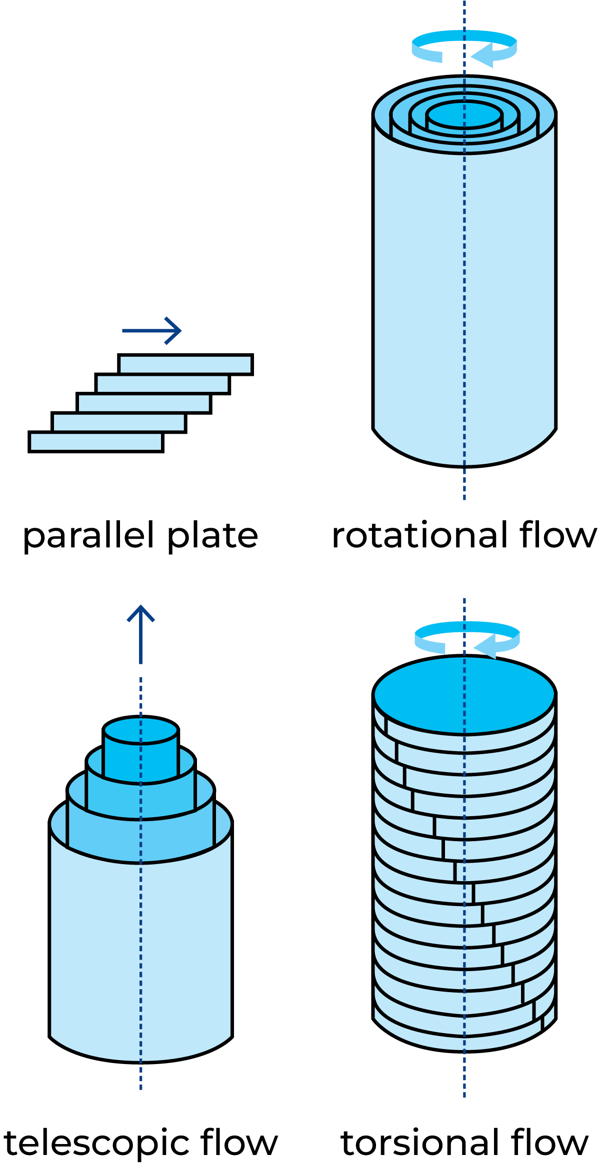
Fig 3.1 Different types of shearing

In rheology, the shearing of a substance is key to knowledge of flow behaviour and structure. Different types of shearing are shown in Figure 3.1. A sheared flow is achieved through flow between parallel planes, rotational flow between coaxial cylinders where one cylinder is stationary and the other one is rotating, telescopic flow through capillaries and pipes, and torsional flow between parallel plates.

To enable the study of the viscosity of a material, the shearing must induce the stationary flow of the material. The flow occurs through the rearrangement and deformation of particles and the breaking of bonds in the structure of the material.

If there is a desire to study the elasticity (structure) of a material, the shearing must be very gentle so as not to destroy the structure. One way to achieve this is to apply an oscillatory shear to the material, with an amplitude low enough to allow an unbroken structure to be studied.

Shearing between parallel planes is normally used for the basic definition of shear stress and shear rate, shown in Figure 3.2, corresponding to how much deformation is applied to the material and how fast. When an external force (F) is acting on a unit area (A) it will create shear flow and its resistance provides the shear stress. How fast the fluid layers move will provide the shear rate. Then the proportionality coefficient between shear stress and shear rate is defined as the apparent viscosity.

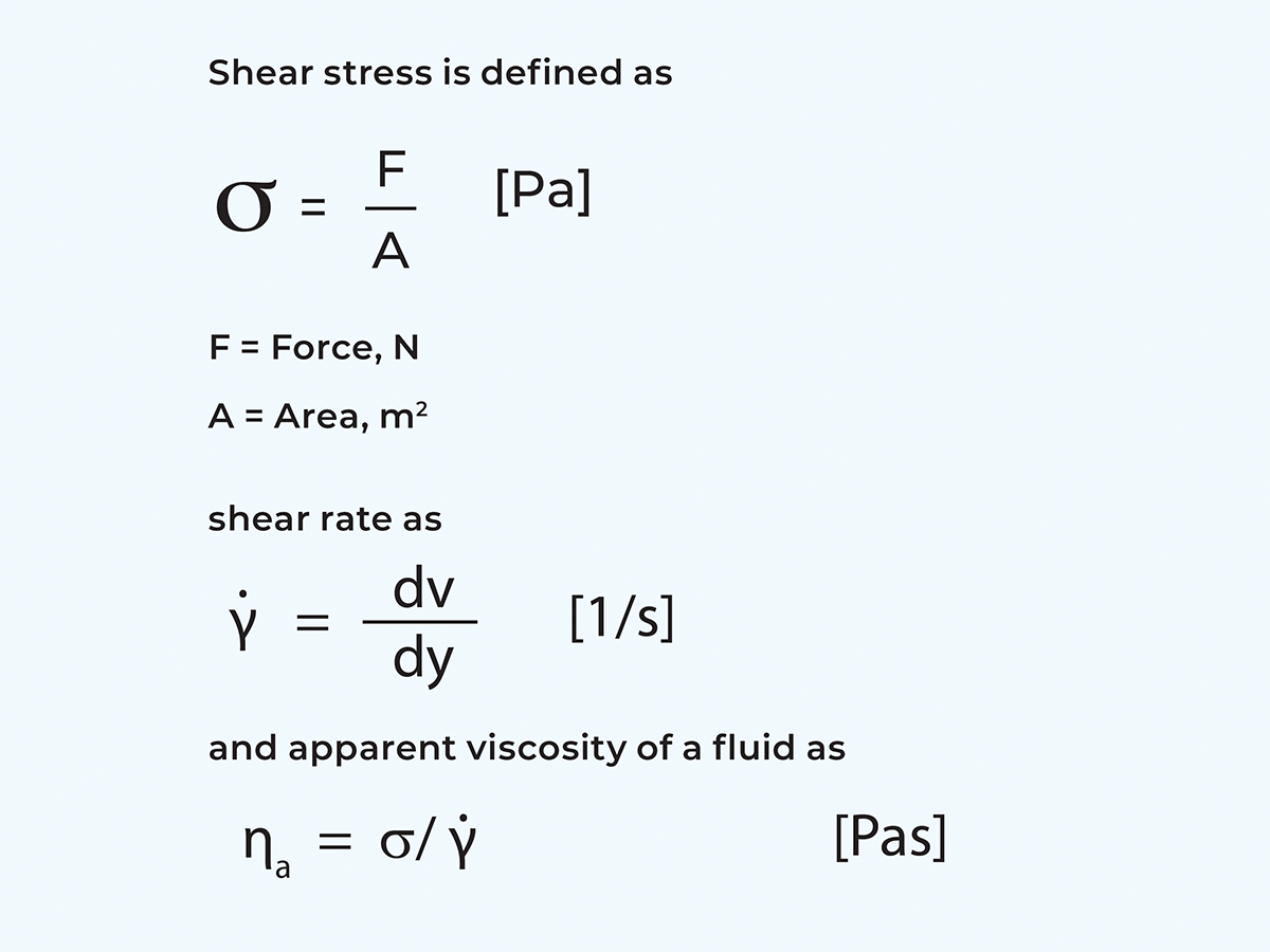
Formula 3.1

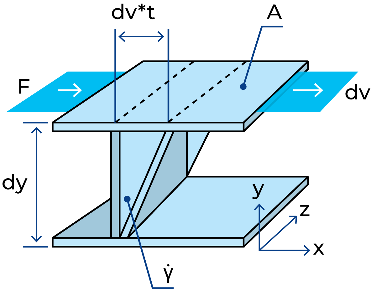
Fig 3.2 Definition of shear stress and shear rate is based on shearing between parallel planes.

Newtonian fluids

Newtonian fluids are those having a constant viscosity dependent on temperature but independent of the applied shear rate. One can also say that Newtonian fluids have a direct proportionality between shear stress and shear rate in a laminar flow.

Formula 3.2

The proportionality constant is thus equal to the viscosity of the material. The flow curve (as shown in Figure 3.3) which is a plot of shear stress versus shear rate, is therefore a straight line with slope for a Newtonian fluid. The viscosity curve (as shown in Figure 3.4), which is a plot of viscosity versus shear rate, is a straight line at a constant value equal to η.

A Newtonian fluid can therefore be defined by a single viscosity value at a specified temperature. Water, mineral and vegetable oils and pure sucrose solutions are examples of Newtonian fluids. Low-concentration liquids in general, such as whole milk and skim milk, may for practical purposes be characterised as Newtonian fluids.

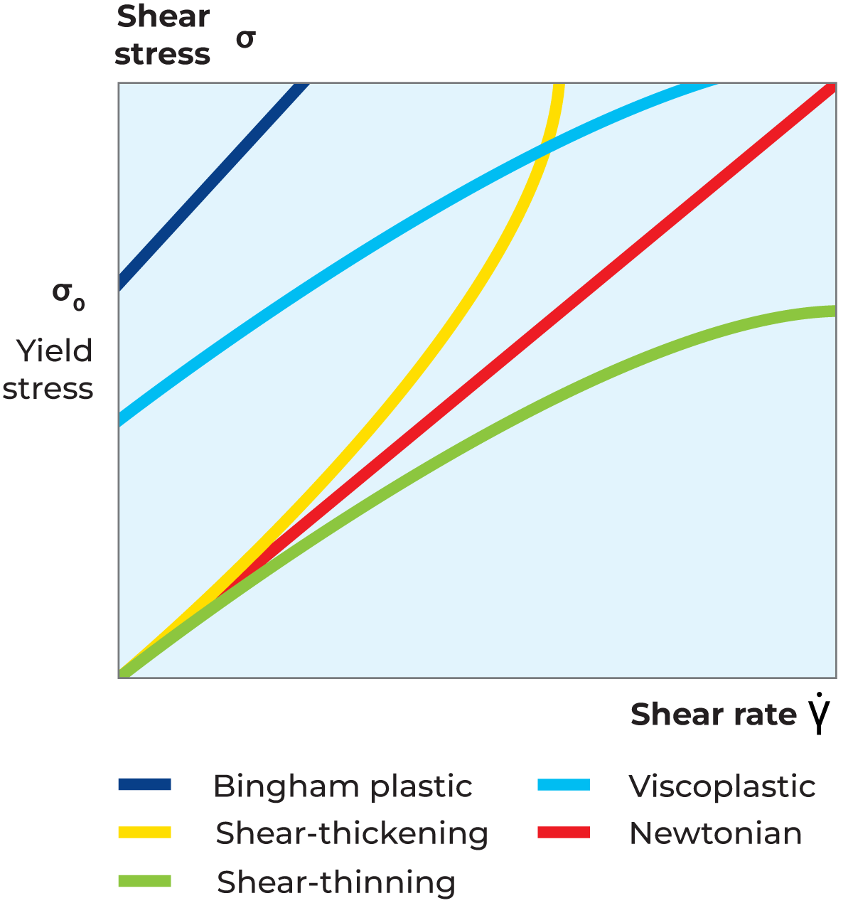
Fig 3.3 Flow curves for Newtonian and non-Newtonian fluids.

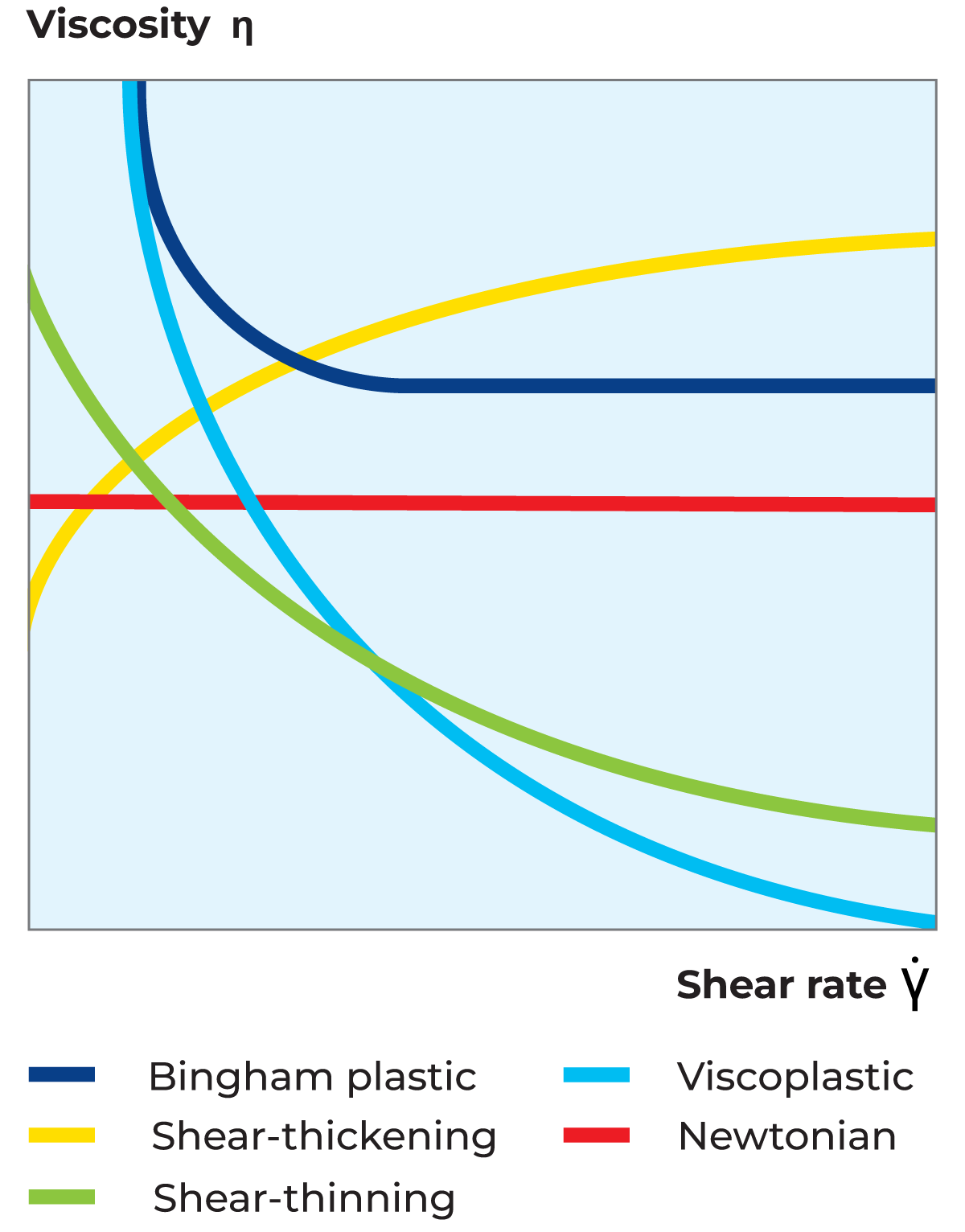
Fig 3.4 Viscosity curves for Newtonian and non-Newtonian fluids.

Non-Newtonian fluids

Materials which cannot be defined by a single viscosity value at a specified temperature are called non-Newtonian. The viscosity of these materials must always be stated together with a corresponding temperature and shear rate. If the shear rate is changed, the viscosity will also change. Generally speaking, high concentrations and low temperatures increase non-Newtonian behaviour.

Apart from being shear-rate dependent, the viscosity of non-Newtonian fluids may also be time-dependent, in which case the viscosity is a function not only of the magnitude of the shear rate but also of the duration and, in most cases, of the frequency of successive applications of shear. Non-Newtonian materials that are time-independent are defined as shear-thinning, shear-thickening or plastic. Non-Newtonian materials that are time-dependent are defined as thixotropic, rheopectic or anti-thixotropic.

Shear-thinning flow behaviour

The viscosity of a shear-thinning fluid (also known as pseudoplastic fluid) decreases with increasing shear rate. Most liquid food systems belong to this category of fluids. The shear rate dependency of the viscosity can differ substantially between different products, and also for a given liquid, depending on temperature and concentration. The reason for shear thinning flow behaviour is that an increased shear rate deforms and/or rearranges particles, resulting in lower flow resistance and consequently lower viscosity, as shown in Figure 3.4. Furthermore, the flow curve for shear-thinning fluid can be observed in Figure 3.3.

Typical examples of shear-thinning fluids are yoghurt, cream, juice concentrates, and salad dressings. It should be noted that although sucrose solutions show Newtonian behaviour independent of concentration, fruit juice concentrates are often significantly non-Newtonian.

Hence a non-Newtonian fluid like yoghurt or fruit juice concentrate being pumped in a pipe shows decreased apparent viscosity if the flow rate is increased. This means, in practice, that the pressure drop of a non-Newtonian fluid in laminar flow is not directly proportional to the flow rate, as it is for Newtonian fluids in laminar flow.

Shear-thickening flow behaviour

The viscosity of a shear-thickening fluid increases with increasing shear rate as shown in Figure 3.4. Furthermore, the flow curve for shear-thickening fluid is shown in Figure 3.3. This type of flow behaviour is generally found among suspensions of very high concentration. A shear-thickening fluid exhibits dilatant flow behaviour, i.e. the solvent acts as a lubricant between suspended particles at low shear rates but is squeezed out at higher shear rates, resulting in a denser packing of the particles. Typical examples of shear-thickening systems are wet sand and concentrated starch suspensions.

Plastic flow behaviour

A fluid that exhibits a yield stress is called a plastic fluid. The practical result of this type of flow behaviour is that a significant force must be applied before the material starts to flow like a liquid. This is often referred to as 'the ketchup effect'. If the force applied is smaller than the force corresponding to the yield stress, the material stores the deformation energy, i.e. shows elastic properties and hence behaves as a solid. Once the yield stress is exceeded, the liquid can flow like a Newtonian liquid and be described as a Bingham plastic liquid, or it can flow like a shear-thinning liquid and be described as a viscoplastic liquid. Both Bingham and viscoplastic curves are shown in Figure 3.3 and Figure 3.4. Typical plastic fluids are quark, high-pectin pineapple juice concentrate, tomato paste and certain ketchups. Outside the liquid food world, toothpaste, hand cream and greases are typical examples of plastic fluids.

A simple but still very effective way of checking a fluid’s possible plastic properties is to just turn the jar upside down. If the fluid does not flow by itself, it probably has a significant yield value. If it flows by itself, but very slowly, it probably has no yield value but a high viscosity. Information of this kind is vital to the design of processing plants, particularly concerning the dimensions and layout of storage and process tank outlets, as well as pump connections.

Time-dependent flow behaviour

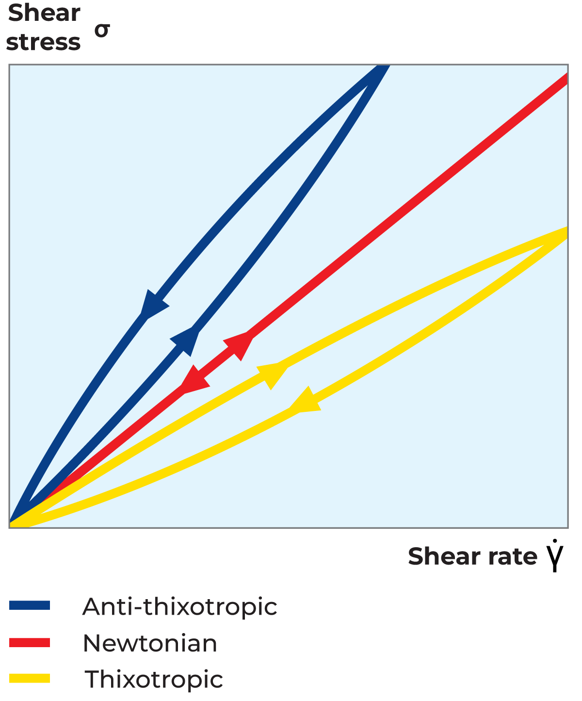
Fig 3.5 Flow curves for time-dependent non-Newtonian fluids.

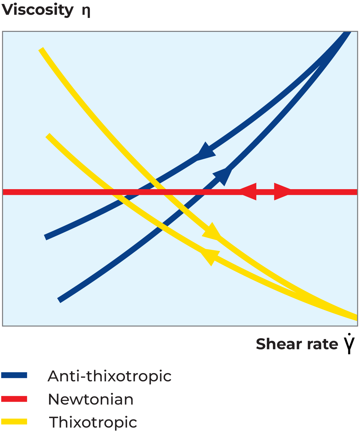
Fig 3.6 Viscosity curves for time-dependent non-Newtonian fluids.

Thixotropic fluids

A thixotropic fluid can be described as a shear-thinning system where the viscosity decreases not only with an increasing shear rate but also with time at a constant shear rate. Thixotropic flow behaviour is normally studied in a loop test. In this test, the material is subjected to increasing shear rates followed by the same shear rates in decreasing order, as shown in the flow curve in Figure 3.5 and the viscosity curve in Figure 3.6. The time-dependent thixotropic flow behaviour is seen from the difference between the ascending and descending viscosity and shear stress curves. To recover its structure, the material must rest for a certain period of time which is characteristic of the specific material. This type of flow behaviour is shown by all gel-forming systems. Typical examples of thixotropic fluids are yoghurt, mayonnaise, margarine, ice cream and brush paint.

Rheopectic fluids

A rheopectic fluid can be described as a thixotropic fluid but with the important difference that the structure of the fluid will only recover completely if subjected to a small shear rate. This means that a rheopectic fluid will not rebuild its structure at rest.

Anti-thixotropic fluids

An anti-thixotropic fluid can be described as a shear-thickening system, i.e. one where the viscosity increases with increasing shear rate, but also with time at a constant shear rate. As with thixotropic fluids, the flow behaviour is illustrated by a loop test and will provide a flow curve, as shown in Figure 3.5, and a viscosity curve, as shown in Figure 3.6. This type of flow behaviour is very uncommon among food products.

Flow behaviour models

For the adaptation of viscosity measurement data to process design calculations, some kind of mathematical description of the flow behaviour is required. For that purpose, several models are available for mathematical description of the flow behaviour of non-Newtonian systems. Examples of such models are Ostwald, Herschel-Bulkley, Steiger-Ory, Bingham, Ellis and Eyring. These models relate the shear stress of a fluid to the shear rate, thus enabling the apparent viscosity to be calculated, as always, as the ratio between shear stress and shear rate.

By far the most general model is the Herschel-Bulkley model, also called the generalised power law equation, which in principle is an extended Ostwald model. The main benefit of the generalised power law equation is its applicability to a great number of non-Newtonian fluids over a wide range of shear rates. Furthermore, the power law equation lends itself readily to mathematical treatment, for instance in pressure drop and heat transfer calculations.

The generalised power law equation is applicable to plastic as well as shear-thinning and shear-thickening fluids according to the following:

Formula 3.3

where:
σ = shear stress, Pa
σ₀ = yield stress, Pa
K = consistency coefficient, Pasⁿ
γ = shear rate, s^–1
n = flow behaviour index, dimensionless

For Newtonian fluids, the generalised power law equation can be written as (with σ = 0, K = hand n = 1):

Formula 3.4

For a shear-thinning or shear-thickening fluid, the generalised power law equation is expressed as:

Formula 3.5

with n < 1 and n > 1, respectively.
Figure 3.7, demonstrates how to calculate both the consistency coefficient (K-value) as well as flow behaviour index from a flow curve. The flow behaviour index (n-value) is calculated from the slope of the flow curve and the consistency coefficient is calculated as shear stress value when shear rate is equal to 1.

For a plastic fluid, the generalised power law equation is used in the fully generalised form, with n < 1 for viscoplastic behaviour and n = 1 for Bingham plastic behaviour.

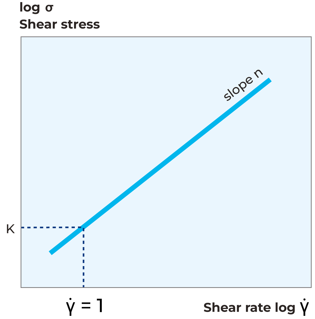
Fig 3.7 Logarithmic flow and viscosity curves for a shear-thinning power-law fluid.

For time-dependent fluids, which in practice means thixotropic fluids, the mathematical models required for the description of rheological behaviour are generally far more complex than the models discussed so far. These fluids are therefore often described by time-independent process viscosities normally fitted to the power law equation.

Typical data

Some typical data on shear rates, viscosities, power law constants (n and K values), and yield stress values at around room temperature (with the exception of molten polymers and molten glass), are shown in Table 3.1.

The unit of viscosity is Pas (Pascal second), which is equal to 1,000 mPas or 1,000 cP (centipoise). Please note also that all viscosity figures should be regarded as examples only (around room temperature) and should NOT be used for calculations.

Measuring equipment

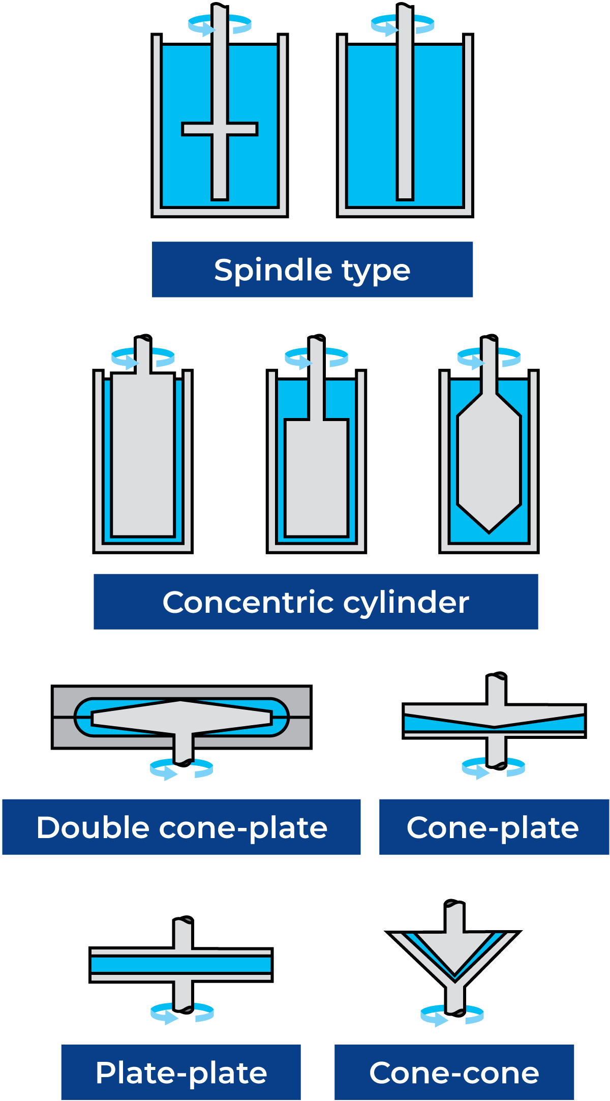
Fig 3.8 Operating principles of different types of rotational viscometers.

The main types of viscometers are rotational and capillary. Rotational viscometers are of the spindle, cone-plate, plate-plate or concentric cylinder type as shown in Figure 3.8. The latter may be of the Searle (rotating bob) or Couette (rotating cup) type. Capillary viscometers may be of the atmospheric or pressurised type. Generally speaking, rotational viscometers are easier to use and more flexible than capillary viscometers. On the other hand, capillary viscometers are more accurate at low viscosities and high shear rates. However, for practical use in liquid food viscometry, they are less applicable due to their sensitivity to even small particles like fruit juice fibres.

Instead, a special design of the capillary viscometer is the tubular viscometer, with a diameter of, e.g. 25 or 38 mm compared to a few mm for the capillary type. The tubular viscometer is used for the determination of the power law constants and is especially suitable for particulate products. The drawbacks of the tubular viscometer are that it often requires large product volumes and the measuring system can be quite bulky and expensive.

Measurement of non-Newtonian fluids requires instruments where the applied shear rate is accurately defined, i.e. where the shearing takes place in a narrow gap with a small shear rate gradient. This important requirement excludes viscometers where the gap is too big or even undefined as it is in viscometers of spindle type, e.g. Brookfield. Furthermore, a single-point instrument or measurement is not suitable for non-Newtonian fluids as it does not provide information about the flow behaviour. It must also be strongly emphasised that viscosity measurements of non-Newtonian fluids carried out at undefined or out-of-range shear rates should not be used as a basis for quantitative analysis of viscosity figures or rheological parameters.

DIN (Deutsches Institut für Normung) is a standardization organisation that defines requirements and standards for specifically dealing with the measurement of viscosities and flow curves using rotational viscometers.

So, to ensure consistent, comparable and absolute viscosity results (which can be used for process design), one should use DIN systems. Some examples of absolute measuring geometries include concentric cylinder (CC), cone-and-plate (CP), and parallel-plate (PP). These geometries allow the calculation of absolute viscosity values independently of the specific measuring geometry used.

Rotational viscometers are available as portable as well as stationary instruments. Portable types usually come in a shockproof case equipped with all necessary accessories. They are basically manually operated, although some manufacturers provide connections for use with personal computers. Today many portable instruments are equipped with processors capable of running a viscometer according to the desired scheme and storing all measuring data for later download to a printer or a PC.

Stationary installations are normally computer-controlled for the automation of measuring sequences and data evaluation. The software usually includes options for fitting to several rheological models, plotting flow curves, and more. A rotational viscometer is normally insufficient for carrying out a complete rheological analysis, for instance, the determination of structure breakdown in yoghurt. This type of analysis requires a more sophisticated instrument, generally called a rheometer. With a rheometer, operating with torsional vibration or oscillation rather than rotation, the fluid can be rheologically analysed without its structure being destroyed.

A typical oscillating flow curve is shown in Figure 3.9. Typical applications are viscoelastic fluids, for which a rheometer can be used to determine the viscous and elastic properties of the fluid separately.

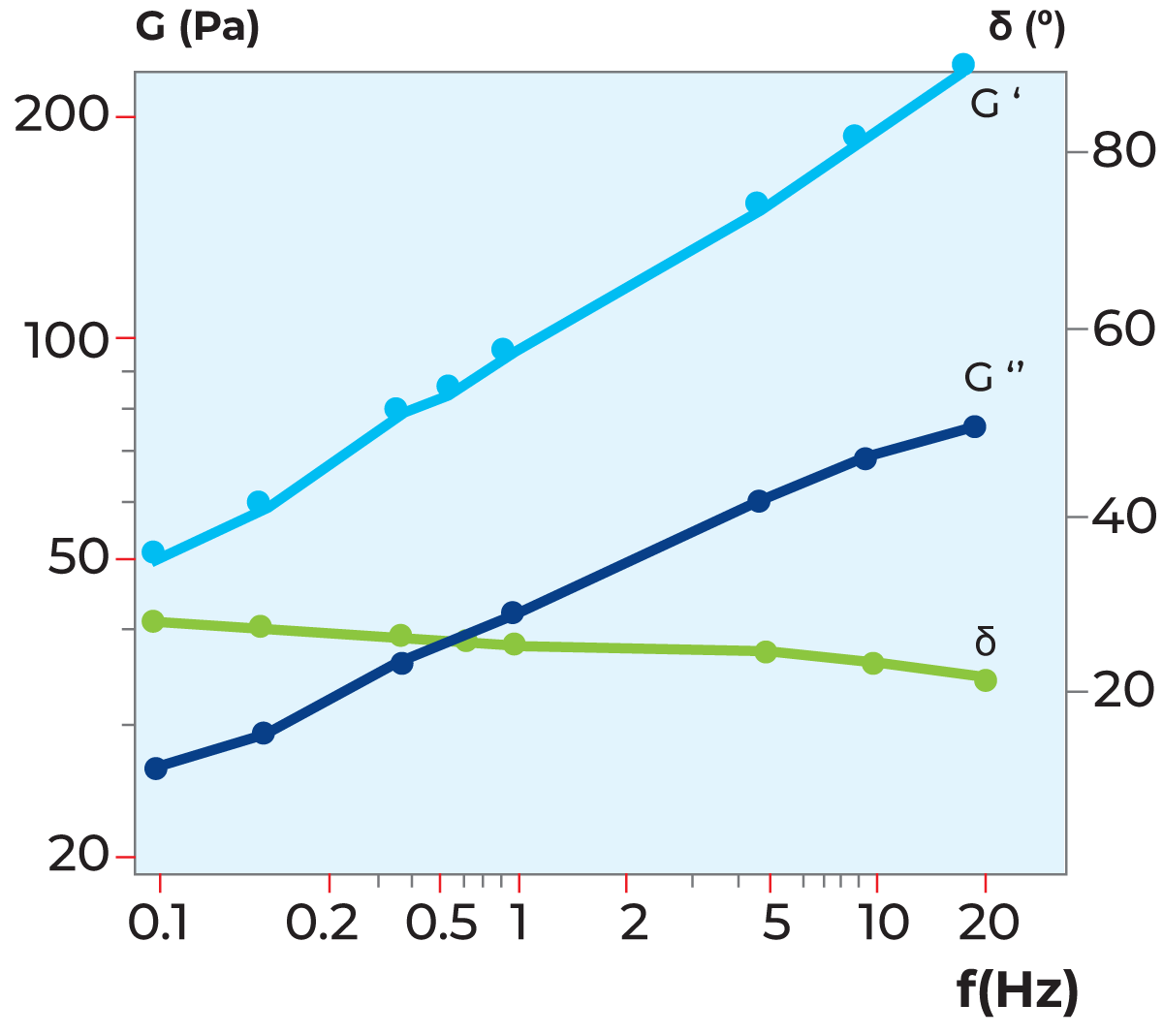
Fig 3.9 Example of an oscillating flow curve.

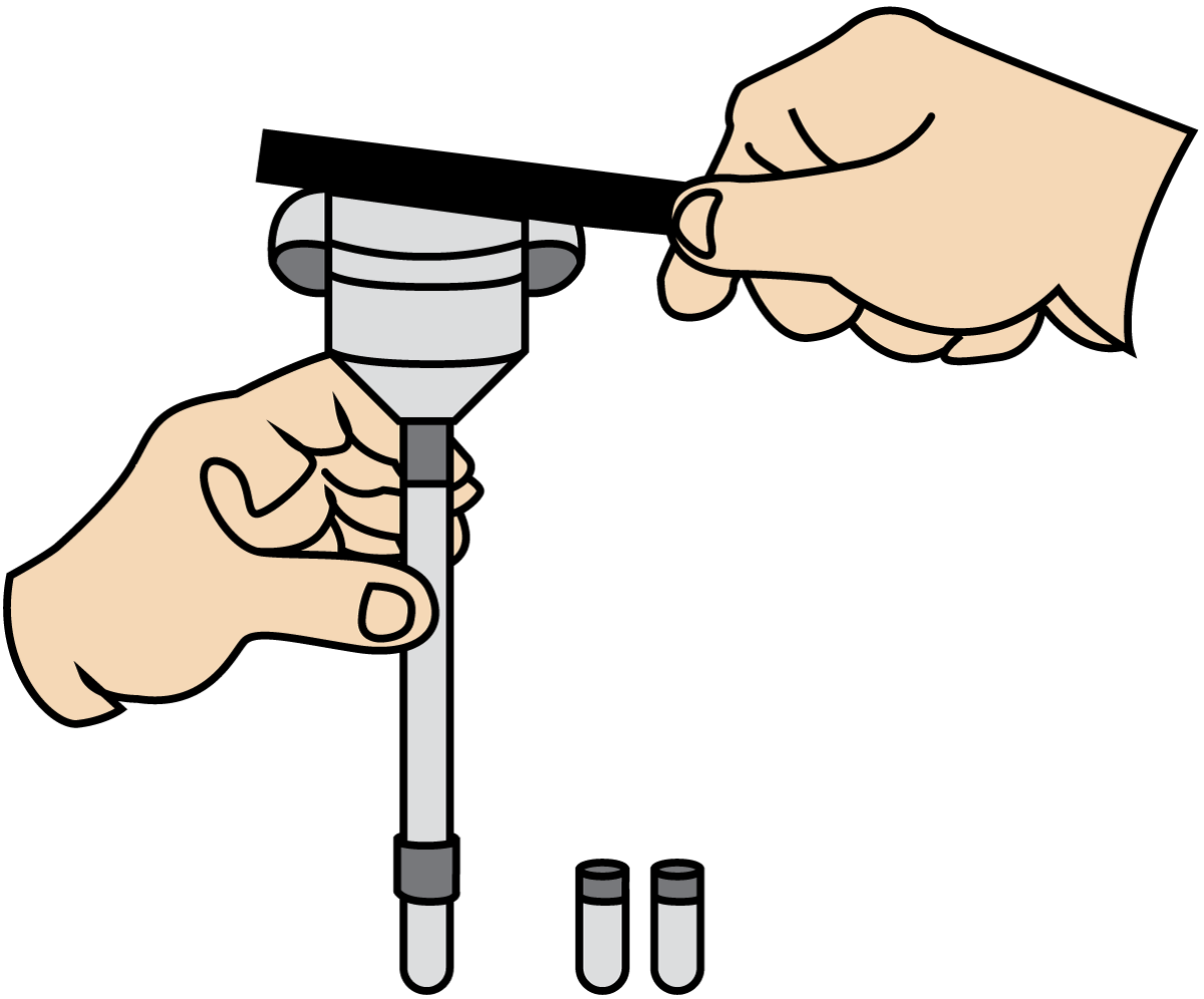
Fig 3.10 The SMR viscometer.

Ordinary viscometers and rheometers should not be used for the measurement of substances with very high viscosities, such as butter, cheese and vegetable fats. Instead, certain types of penetrometers are available, but these cannot be used to obtain scientific rheological results since a penetrometer gives only empirical information that can be used for quality checks.

One special type of consistometer is preferably used within the tomato industry. This type of instrument gives the result in so-called Bostwick degrees, which is a unit applicable only to the comparison of different products. Another type of consistency, used for cream and fermented milk products, is the SMR viscometer at 20 °C, as shown in Figure 3.10, with exchangeable nozzles with a diameter of 2 – 6 mm. The viscosity is reported by specifying the time it takes for a 100 ml sample to flow through a nozzle of a certain diameter.

Measuring techniques

Viscosity measurements should always be carried out for a representative range of shear rates and temperatures related to the process to be studied. The intended use of the measured data should therefore be considered before measuring takes place, for instance, if the viscosity data are to be used in the design of a deep cooler or the heating section of a steriliser.

Due to practical limitations, the maximum applicable temperature for most viscometers is around 90 °C. At higher temperatures, the risk of evaporation from the surface of the test sample, followed by skin formation leading to increased momentum and hence false readings, is significant. Hence, a special type of pressurised measuring system has to be employed. With these systems, temperatures up to 150 °C are possible, i.e. a typical sterilisation process up to 140 °C can be fully covered regarding viscosity data. It is also most important that the temperature is kept constant during the test period and, of course, that it is accurately measured. A temperature change of 3 °C can often cause a change in viscosity of 10%.

To increase the accuracy of data evaluation, measurements should be made at as many different shear rates and temperatures as possible. In addition, heating effects must be considered. In a substance containing hot-swelling starch, for example, the viscosities before and after heating above swelling temperature will differ significantly. For that reason, it makes sense to analyse these types of products both before and after gelatinisation.

Furthermore, storage conditions and time factors must be taken into consideration. The rheological properties of many products, e.g. fermented dairy products, change with time. If the purpose of the viscosity measurement is to supply data for process design, the measurements should preferably be made in as close a connection as possible to the actual processing stage. It might be necessary to consider analysing the food products directly at the customer site to obtain proper data for design purposes.

When measurements are performed on a regular basis, the results are preferably stored in a database to facilitate comparison of various products. In practice, all varieties of liquid food products are unique regarding viscosity data, meaning that data measured on one type of vanilla pudding, one type of tomato purée or one type of yoghurt cannot be safely applied to another type or brand of product with the same name or even with roughly the same composition. However, with access to a database containing data on a substantial number of products, there is always a possibility to extract a range of viscosities for a certain type of product in case no other information is available.

Pressure drop calculations

Some useful equations are given below for the manual calculation of pressure drop and shear rates for flow in circular and rectangular channels. All equations are based on the power law expression, as most food systems in processing conditions can be described by this expression.

The equations are applicable to Newtonian as well as non-Newtonian fluids, depending on the value of n used in the calculation: n < 1 for shear-thinning (pseudoplastic) fluids, n = 1 for Newtonian fluids, and n > 1 for shear-thickening (dilatant) fluids.

The relationship between flow rate and pressure drop and between flow rate and wall shear rate in a circular channel is described as follows:

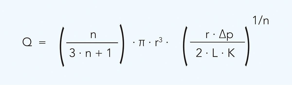
Formula 3.6

or

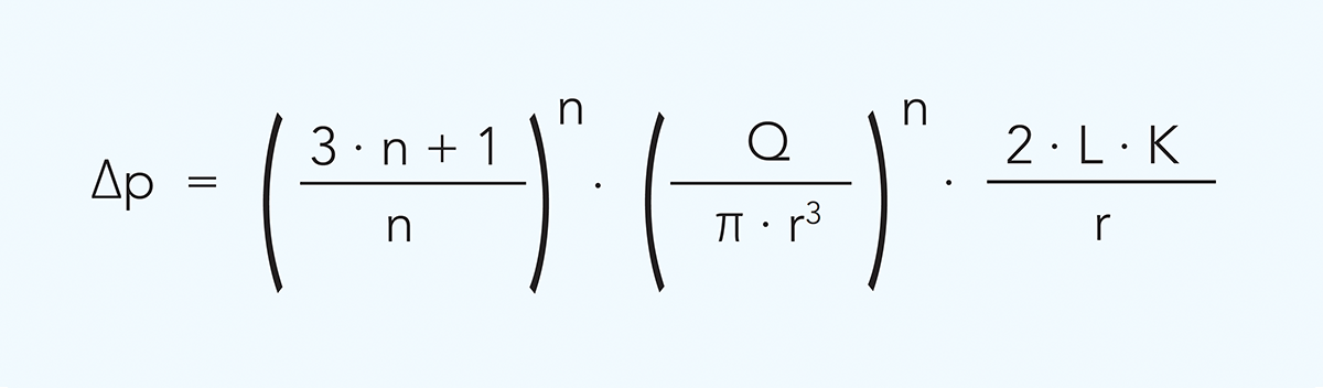
Formula 3.7

and

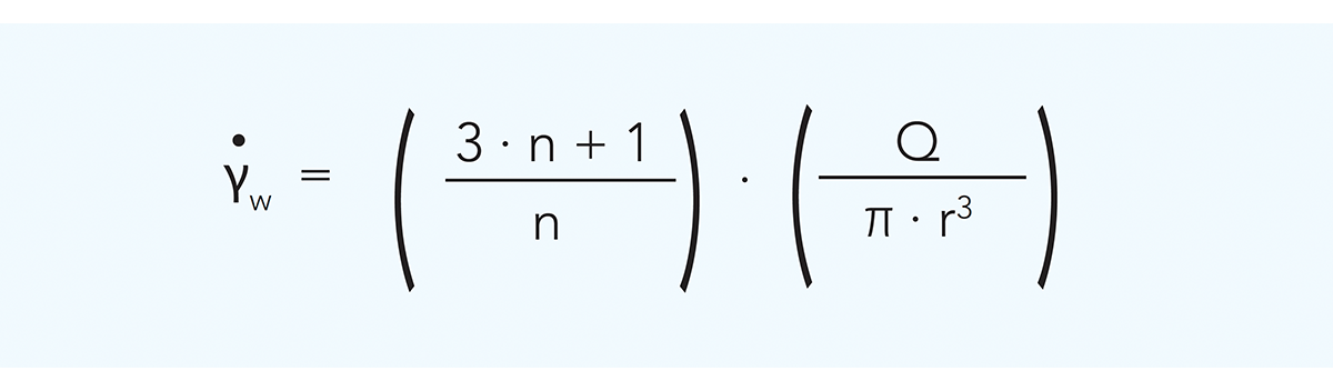
Formula 3.8

The corresponding equations for rectangular channels are as follows:

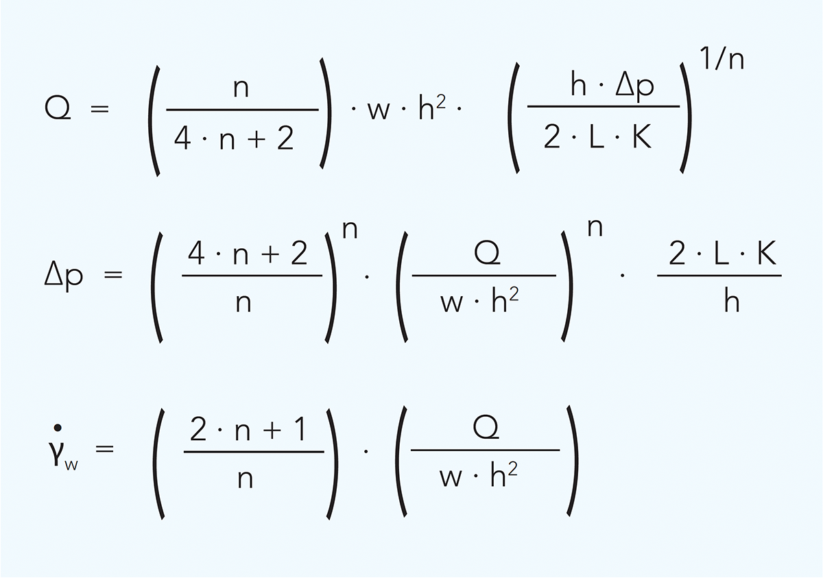
Formula 3.9